Survival Analysis in Cricket
Survival Analysis
Survival analysis deals with estimating probability of continuation of a particular status-quo at given point in time. Naturally, it also estimates the probability of discontinuation of the status quo i.e. occurrence of an event or a hazard. It finds application in several fields. For e.g. in medicine to estimate probability of survival of a patient under treatment of a fatal disease. Or in engineering to estimate reliability or predicting failure. Even in marketing and sales, for e.g. to decrease churn rate.
Cricket
In this piece, application of similar method in the game of cricket has been illustrated. Survival in this case means 'not getting out or dismissed' while batting. Naturally hazard means getting out. ODI Batting statistics of two Indian batsmen have been used. They are Sachin Tendulkar and Sourav Ganguly. Data has been sourced from ESPN.
 1#data frames named ganguly and tendulkar are loaded
 2
 3#function to manipulate data
 4mani<-function(x){
 5x<-x%>%
 6  filter(Pos != "-")%>%
 7  mutate(diss=ifelse((Dismissal=="not out"),0,1))%>%    #This is the event of interest
 8  mutate(Runs=str_remove(Runs,"[*]"))%>%
 9  mutate(BF=as.integer(BF), Runs=as.integer(Runs),
10         Mins=as.integer(Mins),Fours=as.integer(Fours),Sixes=as.integer(Sixes),
11         SR=as.numeric(SR),Pos=as.integer(Pos),
12         Dismissal=as.factor(Dismissal), Inns=as.factor(Inns),
13         Date=dmy(Date))%>%
14  separate(Opposition,c(NA,"Opposition"),extra = "merge", fill = "left")%>%
15  separate(Ground,c(NA,"Ground"),extra = "drop", fill = "left")%>%
16  mutate(Runs=ifelse(is.na(Runs),round(BF*SR,0),Runs))%>%   #BF or Balls Faced will be used as unit of time
17  mutate(h_cen=ifelse((Runs>=50 & Runs<100),1,0))%>%
18  mutate(cen=ifelse(Runs>=100,1,0))
19#Adding dummy columns for possible future requirement
20#x<-dummy_cols(x,select_columns = c("Opposition","Ground"))
21return(x)
22}
23
24#Adding player names in their data sets
25
26ganguly$player<-c(rep("ganguly",nrow(ganguly)))
27tendulkar$player<-c(rep("tendulkar",nrow(tendulkar)))
28
29#Combining data of the three players
30
31data.raw<-rbind(ganguly,tendulkar)
32
33#structuring the data using the function created
34
35data.df<-mani(data.raw)
36head(data.df)
 1##   Runs Mins BF Fours Sixes     SR Pos Dismissal Inns  X  Opposition     Ground
 2## 1    3   33 13     0     0  23.07   6       lbw    1 NA West Indies   Brisbane
 3## 2   46  117 83     3     0  55.42   3   stumped    1 NA     England Manchester
 4## 3   16   NA 41     3     0  39.02   3    caught    1 NA   Sri Lanka        RPS
 5## 4   36   59 52     3     1  69.23   3    caught    2 NA    Zimbabwe        SSC
 6## 5   59  102 75     7     0  78.66   7       lbw    1 NA   Australia        SSC
 7## 6   11   NA  8     1     0 137.50   8   not out    1 NA    Pakistan    Toronto
 8##         Date  player diss h_cen cen
 9## 1 1992-01-11 ganguly    1     0   0
10## 2 1996-05-26 ganguly    1     0   0
11## 3 1996-08-28 ganguly    1     0   0
12## 4 1996-09-01 ganguly    1     0   0
13## 5 1996-09-06 ganguly    1     1   0
14## 6 1996-09-17 ganguly    0     0   0
Estimating probability of staying 'not out'
Kaplan Meier Analysis is a non-parametric analysis. This means that only the event and the time is used in the analysis i.e. for e.g. possible effect of Opposition will not be considered. Unless, of course the data is grouped based on a parameter. Just like we will group the data based on players so that we observe the survival statistics for the individual players. We can further group the data based on Opposition or Ground.
1kap.mr.fit<-survfit(Surv(BF,diss) ~ player, data=data.df)
2summary(kap.mr.fit)$table
1##                  records n.max n.start events   *rmean *se(rmean) median
2## player=ganguly       300   300     300    279 53.35585   2.532818     41
3## player=tendulkar     318   318     318    278 52.39229   2.131667     44
4##                  0.95LCL 0.95UCL
5## player=ganguly        32      45
6## player=tendulkar      38      56
Detailed summary can viewed by running 'summary(kap.mr.fit)'.
The results do not show any significant difference in the survival tendencies of the two batsmen, yet. Plotting the data makes this clear.
 1ggsurvplot(
 2  kap.mr.fit,
 3  pval = TRUE, # show p-value
 4  break.time.by = 25, #break X axis by 25 balls
 5  #risk.table = "abs_pct", # absolute number and percentage at risk
 6  #risk.table.y.text = FALSE,# show bars instead of names in text annotations
 7  linetype = "strata",
 8  # Change line type by groups
 9  conf.int = TRUE,
10  # show confidence intervals for
11  #conf.int.style = "step",  # customize style of confidence intervals
12  surv.median.line = "hv",
13  # Specify median survival
14  ggtheme = theme_bw(),
15  # Change ggplot2 theme
16  legend.labs =
17    c("Ganguly", "Tendulkar"),
18  # change legend labels
19  ncensor.plot = TRUE,
20  # plot the number of censored subjects (outs) at time t
21  #palette = c("#000000", "#2E9FDF","#FF0000")
22)+
23  labs(x="Balls")
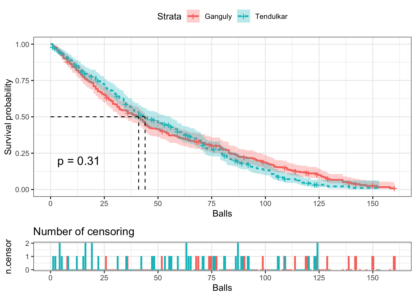
Survival probabilities of both are almost similar. The survival probability of Ganguly at the beginning of the innings is slightly lower than that of Tendulkar. However, after around 75 balls, it increases and exceeds than that of Teldulkar. But the difference is insignificant.
Estimating probability of Sixers
Similar approach was used to estimate probability of at least one sixer. The event, or hazard (for the fielding team) is the batsman hitting a sixer. The hazard plot reveals interesting insight.
 1#creating new data set with result of sixes
 2data.new<-data.df%>%
 3  mutate(six=ifelse(Sixes>0,1,0))
 4
 5#fitting the model
 6kap.six.fit<-survfit(Surv(BF,six) ~ player, data=data.new)
 7
 8#summary(kap.six.fit)$table
 9ggsurvplot(
10  kap.six.fit,
11  pval = TRUE,
12  break.time.by = 25,
13  linetype = "strata",
14  conf.int = TRUE,
15  surv.median.line = "hv",
16  ggtheme = theme_bw(),
17  legend.labs =
18    c("Ganguly", "Tendulkar"),
19  ncensor.plot = TRUE,
20  fun = "event"
21)+
22  labs(x="Balls", y="Sixer")
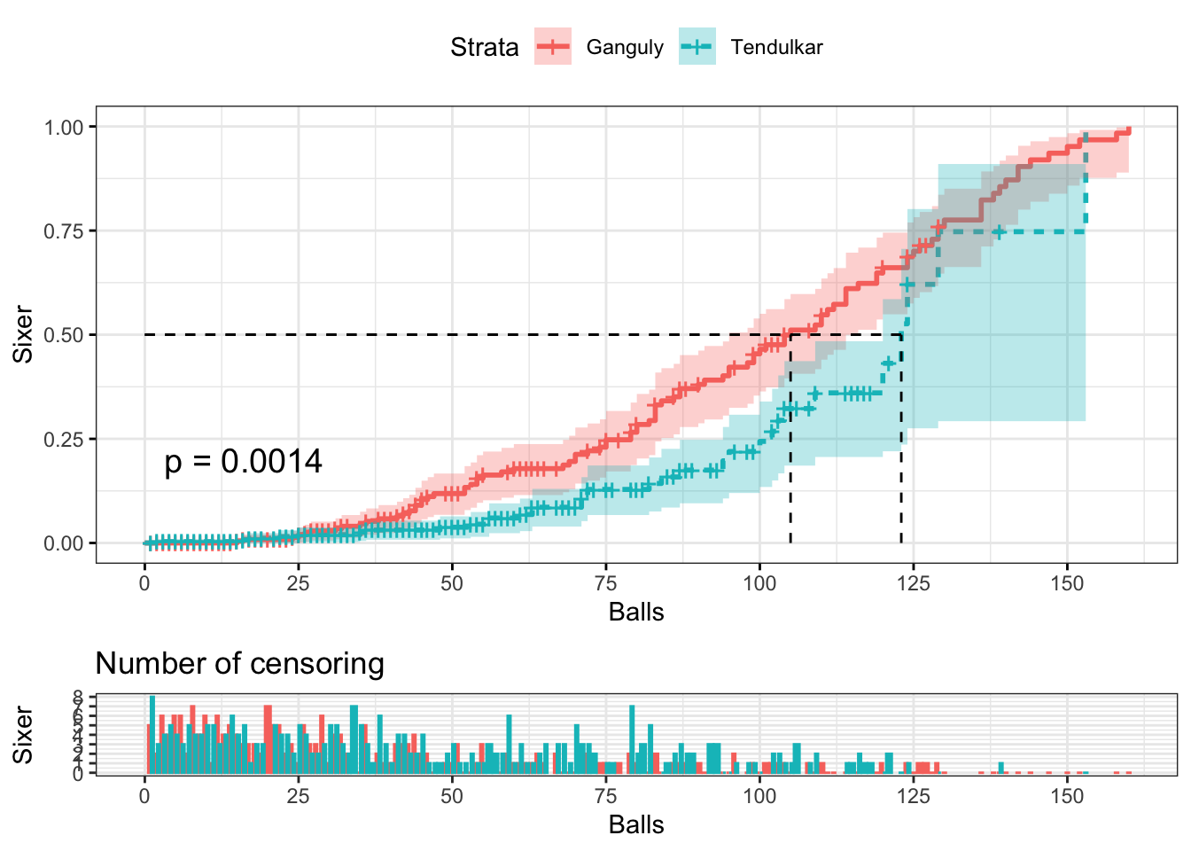
The result clearly shows why Ganguly was a 'Hazard' for the fielding team after he had set in. The probability of him hitting at least one sixer is substantially higher than that of Tendulkar, esp. after 40 balls or so. The narrow strip of confidence interval indicates higher accuracy in the estimate, in case of Ganguly. The confidence interval spreads wide in case of Tendulkar, indicating higher uncertainty in estimates.
Similar analysis was conducted using Cox Proportional Hazard model. This model is capable to consider effect of other parameters. 'Runs' was used as another parameter in the new model and the hazard plot was plotted again.
1cox.fit <- survfit(coxph(Surv(BF, six) ~ Runs + strata(player),
2                         data = data.new))
3autoplot(
4  cox.fit,
5  fun = 'event',
6  censor = FALSE,
7  conf.int = TRUE,
8  surv.linetype = 'strata'
9)+ labs(x = "Balls", y = "Sixer")
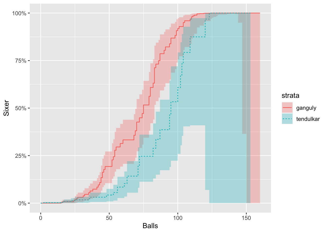
The results are similar. The probability of sixer by Ganguly is substantially higher than that of Tendulkar esp. from around 25 balls to around 120 balls. The confidence interval widens in the right end of the curve, indicating immense uncertainty.
Final Analyses
The final stage of analysis includes a subset of the data previously used. Specifically, a few 'Opposition' was selected with whom the number of matches were substantially higher than the rest.
 1#Defining the opposition teams
 2
 3teams<-c("Pakistan","Sri Lanka", "Australia", "West Indies", "South Africa", "New Zealand",
 4"Zimbabwe", "England", "Kenya", "Bangladesh")
 5
 6#Creating new data set with by filtering the teams
 7data.new<-data.new%>%filter(Opposition %in% teams)
 8
 9# Fitting Cox models
10
11#Sixes
12cox.six<-survfit(coxph(Surv(BF,six) ~ Runs+strata(player)+factor(Opposition),
13                    data = data.new))
14sixerplot<-autoplot(cox.six,conf.int = TRUE,fun='event',pval=TRUE)+labs(x="Balls",y="Sixer Chance")+theme(legend.position = "top")
15
16#Dismissals
17cox.diss<-survfit(coxph(Surv(BF,diss) ~ Runs+strata(player)+factor(Opposition),
18                    data = data.new))
19dissplot<-autoplot(cox.diss,conf.int = TRUE,pval=TRUE)+labs(x="Balls",y="Survival Chance")+theme(legend.position = "top")
20
21#Half centuries
22cox.hcen<-survfit(coxph(Surv(BF,Runs>=50) ~ strata(player)+factor(Opposition),
23                    data = data.new))
24hcenplot<-autoplot(cox.hcen,conf.int = TRUE, fun='event',
25         pval=TRUE,plotTable = TRUE, divideTime = 25,)+labs(x="Balls",y="Chance of half century")+xlim(50,100)+theme(legend.position = "top")
26
27#Result of Dismissal
28cox.diss
1## Call: survfit(formula = coxph(Surv(BF, diss) ~ Runs + strata(player) +
2##     factor(Opposition), data = data.new))
3##
4##             n events median 0.95LCL 0.95UCL
5## ganguly   292    273     44      42      51
6## tendulkar 313    276     53      45      59
1#Result of Sixes
2cox.six
1## Call: survfit(formula = coxph(Surv(BF, six) ~ Runs + strata(player) +
2##     factor(Opposition), data = data.new))
3##
4##             n events median 0.95LCL 0.95UCL
5## ganguly   292     92     70      54     100
6## tendulkar 313     32     94      72      NA
1#Result of Half Century
2cox.hcen
1## Call: survfit(formula = coxph(Surv(BF, Runs >= 50) ~ strata(player) +
2##     factor(Opposition), data = data.new))
3##
4##             n events median 0.95LCL 0.95UCL
5## ganguly   292     89     90      83     111
6## tendulkar 313     93     82      72      99
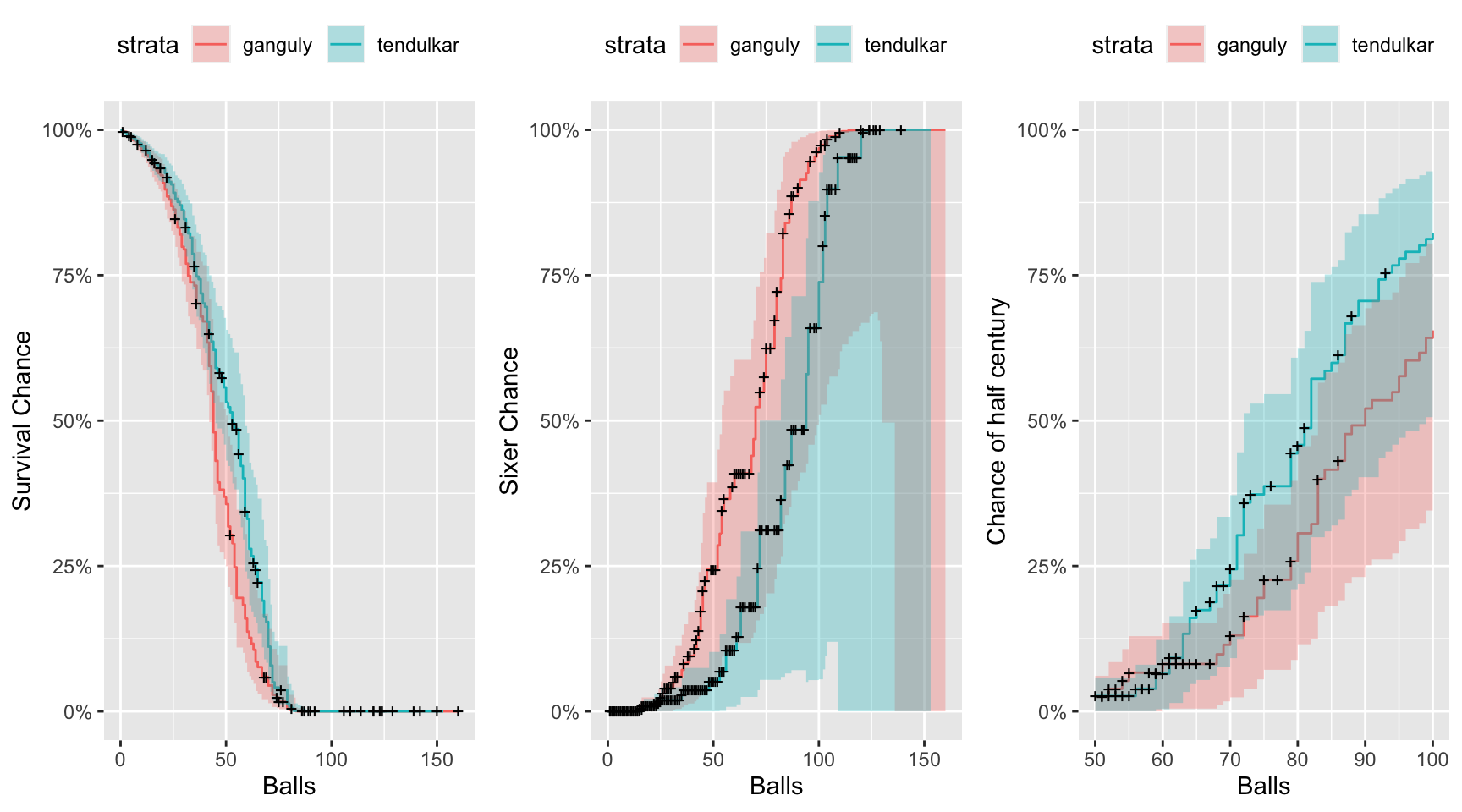
Results:
Tendulkar will remain longer on crease than Ganguly
- Ganguly will be dismissed by the time he faces 44 to 51 balls, about 50% of the time. This should be true 95% of the time.
- Tendulkar will be dismissed by the time he faces 53 to 60 balls, about 50% of the time. This should be true 95% of the time.
Conclusion: Chances are higher that Tendulkar will remain on crease longer than Ganguly.
Ganguly will sixes earlier than Tendulkar
- Ganguly will hit at least one six by the time he faces 70 to 83 balls, 50% of the time. This should be true 95% of the time.
- Tendulkar will hit at least one six by the has faces 87 balls. This should be true 95% of the time.
Conclusion: Chances are higher that on average, Ganguly will hit six much before Tendulkar does, in an innings.
Ganguly will score slower till a point, than Tendulkar
- If Ganguly faces 96 to 111 balls, 50% of the time he will score a half century. This should be true 95% of the time.
- If Tendulkar faces 85 to 99 balls, 50% of the time he will score a half century. This should be true 95% of the time.
Conclusion: Chances are higher that Ganguly will score slower on average that Tendulkar, at least till reaching half century.
The plots of the result are as follows.
1#Plotting and arranging
2ggarrange(dissplot,sixerplot,hcenplot,ncol=3)
Further possibilities
After building any model, the model should be tested on a test data to check for accuracy. Validation of the model is required to understand the robustness of the model. If the results are not satisfactory, changes are made to the model to improve accuracy. The process is repeated a few times on requirement.
The predictions are based on certain parameters. There will be more parameters on which the outcome will depend. For e.g. the above analysis considers opposition team as a parameter. However, the ground and weather will also impact the outcome, which has not been considered. There is always a possibility to add more parameter to improve results.
The effect of parameters may also change over time. For e.g. the opposition team may change members in their team, say, add a fast bowler. Also, the batsmen may evolve themselves to tackle a difficult opponent. Then the effect of the opponent on the outcome will not remain same throughout time. Further complex methods like accelerated failure models can be applied to improve the model.
These are beyond the scope of this article. Feel free to try them out and don't forget to share your results. Feel free to reach out if you need help.
Survival Analysis can be used to help reduce churn, reduce warranty cost and improve pricing, predict failure in machinery and more. If you are curious about how it can help you achieve your business goals, do not hesitate to contact me.