Network analysis in Bollywood
Network Analysis
Network theory is the study of graphs as a representation of relationship between discrete elements. When applied to social relations, it is known as social network analysis.1
Bollywood
In this article, network theory is applied to analyse relationship between some professionals in bollywood, based on data from movie set. The data has been compiled by Parth Parikh from various sources. The analysis in this article involves a subset of relevant data.
Data preparation
The CSVs downloaded are imported as following
- film1: Movie details from 1950 to 1989
- film2: Movie details from 1990 to 2009
- film3: Movie details from 2010 to 2019
- crew: Crew information with unique identifier
- filmcrew: Crew details (unique identifier) in each movie
 1#Combining film data
 2films<-rbind(film1,film2,film3)
 3rm(film1,film2,film3)
 4# separating columns with actor names, since actor names are in single column
 5f<-films%>%
 6  separate(actors,c
 7           ("a1","a2","a3","a4","a5","a6","a7","a8","a9","a10"),sep="[|]")%>%
 8    filter(a1!="NA")
 9#dedup any possible duplicates in movie
10f<-f[!duplicated(f$imdb_id), ]
11rm(films)
12# selecting relevant columns from filmcrew
13fc<-filmcrew[,c(1,2,4,5)]
14rm(filmcrew)
15# separating column with writer names, since writer names are in single column and deleting rows with no writer
16c<-crew%>%
17    separate(writers, c("w1","w2","w3","w4","w5","w6","w7","w8","w9","w10"), sep="[|]")%>%
18    filter(w1!="\\N")
19#dedup any possible duplicates in movie
20c<-c[!duplicated(c$imdb_id), ]
21rm(crew)
22#Compilining actor and crew info per movie together
23full.coded.raw<-c%>%right_join(f,by=c("imdb_id"))
24
25#Relevant columns are directors, writers and actors i.e. director, wx and ax
26dt<-full.coded.raw[,c(2:12,16:25)]
27rm(full.coded.raw)
28#To create a file suitable for network analysis, a 2 column file is required, which depicts relationships. This can be achieved by creating combination of columns and binding them together. It can be done manually or the `juggling_jaguar` function from package `Rmessy` can be used. The package is under development. Please feel free to use it and develop it further. The package can be downloaded from github here. Or it can be installed using devtools using the following command.
29
30#>install.packages("devtools") #if not installed
31#>devtools::install_github("asitav-sen/Rmessy")
32
33#using juggling_jaguar
34
35dt.net<-juggling_jaguar(dt)
36rm(dt)
37
38# names(dt.net)[1]="x"
39# names(dt.net)[2]="y"
40#
41# dt.net<-
42#   dt.net%>%filter(x!=y)
43
44
45
46#The data frame contains unique ids of the crew (and names of the actors). The data frame fc contains the relevant information to get the names of the relevant codes. However, since actor names are not coded, it is important that their names remain intact.
47
48dt.net1<-
49dt.net%>%
50  left_join(fc,by=c("x"="crew_id"))%>%
51  mutate(from=ifelse(is.na(name),x,name))%>%
52  select(c(6,2))%>%
53  left_join(fc,by=c("y"="crew_id"))%>%
54  mutate(to=ifelse(is.na(name),y,name))%>%
55  select(c(1,6))
56rm(dt.net)
57# Since some of the names were not found in the crew list available, these rows may be deleted. This is optional. One may want to analyse using the codes.
58dt.net2<-
59dt.net1%>%
60  filter(!str_detect(to,"^nm"))%>%
61  filter(!str_detect(from,"^nm"))
62rm(dt.net1)
63#Removing possible empty rows
64
65rm.ro<-which(dt.net2$to=="")
66dt.net2<-dt.net2[-rm.ro,]
67
68#In this data set, pair of A-B and B-A are considered different. However, they are ultimately same. Hence, the data was further rectified.
69# converting df in igraph file
70
71gra.ph<-graph_from_data_frame(d=dt.net2, directed=FALSE)
72
73# converting back to data frame
74
75data.df<-get.data.frame(gra.ph)
76rm(gra.ph)
77#To analyze 'strength of relation' one can assume the number of times people have worked together to be a good indicator.
78data.df<-
79  data.df%>%
80  group_by(from,to)%>%
81  count()%>%
82  arrange(desc(n))%>%
83  rename(works=n)%>%
84  filter(from!=to)
85
86# creating graph object and Removing scatters
87
88gra.ph<-graph_from_data_frame(d=data.df, directed=FALSE)
89gra.ph$weight<-data.df$works
90V(gra.ph)$comp <- components(gra.ph)$membership
91gra.main <- induced_subgraph(gra.ph,V(gra.ph)$comp==1)
92rm(gra.ph)
Analyses
Understanding importance of nodes (individuals) and the network
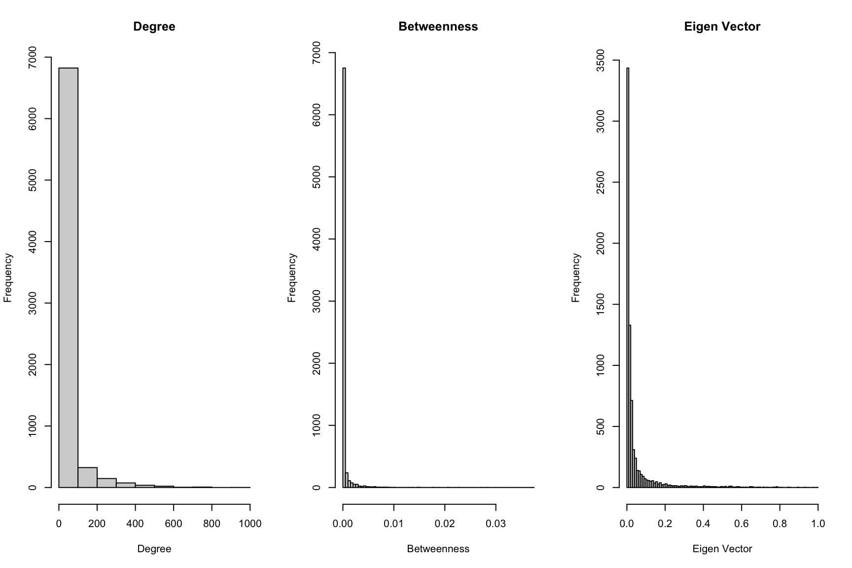
There is immense inequality in the importance of the individuals. Out of all, very few individuals have worked with more than 100 different people in the industry. This is observed through histogram of degrees. Similar trend is observed in the histogram of betweenness, which is another indicator of importance. Roughly, betweenness in this case can be simplified as the tendency to do have worked with different individuals who have not worked together. (This is an oversimplification)
1main.deg<-degree(gra.main, mode = "all")
2main.bw<-betweenness(gra.main,directed = FALSE, normalized = TRUE)
3eigen.main<-eigen_centrality(gra.main)
4par(mfrow=c(1,3))
5hist(main.deg, breaks = 10, main = "Degree", xlab = "Degree")
6hist(main.bw, breaks = 100, main = "Betweenness", xlab = "Betweenness")
7hist(eigen.main$vector, breaks = 100, main= "Eigen Vector", xlab = "Eigen Vector")
The top individuals identified are mentioned in the table.
1bydegree<-sort(main.deg, decreasing=TRUE)[1:20]
2bybetweenness<-sort(main.bw, decreasing=TRUE)[1:20]
3byeigen<-sort(eigen.main$vector,decreasing = TRUE)[1:20]
4
5top<-data.frame(bydegree,bybetweenness,byeigen)
6top
 1##                    bydegree bybetweenness   byeigen
 2## Anupam Kher             904    0.03737696 1.0000000
 3## Gulshan Grover          798    0.02848179 0.9701978
 4## Shakti Kapoor           779    0.02748425 0.9354072
 5## Aruna Irani             773    0.02258863 0.9272276
 6## Prem Chopra             739    0.02089639 0.8935966
 7## Amitabh Bachchan        725    0.02057037 0.8924957
 8## Asrani                  723    0.01898179 0.8523556
 9## Dharmendra              707    0.01789976 0.8479439
10## Mithun Chakraborty      672    0.01777744 0.8417188
11## Om Puri                 657    0.01526129 0.8135059
12## Pran                    633    0.01497864 0.8016672
13## Paresh Rawal            625    0.01481343 0.7927105
14## Amrish Puri             591    0.01458164 0.7898096
15## Jackie Shroff           586    0.01362665 0.7886611
16## Naseeruddin Shah        583    0.01347162 0.7875499
17## Satyendra Kapoor        571    0.01282562 0.7858475
18## Johnny Lever            570    0.01215650 0.7852549
19## Rishi Kapoor            566    0.01104178 0.7800349
20## Jeetendra               565    0.01039253 0.7749431
21## Kader Khan              563    0.01029858 0.7732780


The farthest or the longest connection in the network is between Ajai Sinha and Edwin Fernandes with 5 individuals in between.
1farthest_vertices(gra.main)
1## $vertices
2## + 2/7436 vertices, named, from edb7f57:
3## [1] Ivan Ayr   Adiba Bhat
4##
5## $distance
6## [1] 7
1get_diameter(gra.main)
1## + 8/7436 vertices, named, from edb7f57:
2## [1] Ivan Ayr         Himanshu Kohli   Barkha Madan     Rekha
3## [5] Amitabh Bachchan Prateik          Nitin Kakkar     Adiba Bhat
The assortativity based on degree i.e. tendency for individuals to work with other individuals with similar degree (connections), lies somewhere in the middle, near 0. There is almost equal mix of cases.
1assortativity.degree(gra.main, directed= FALSE)
1## [1] 0.0175864
Transitivity of 0.23 is much higher than that of randomly generated network of similar properties. However, it is not uncommon to observe social networks to have transitivity between 03. to 0.6.2 Transitivity measures how well connected the network is. (Oversimplification)
 1# creating random trees for comparison
 2# *****Requires substantial computational power*****
 3
 4rnd.main <- vector('list',500)
 5dens.main<-edge_density(gra.main)
 6n=gorder(gra.main)
 7
 8for(i in 1:500){
 9  rnd.main[[i]] <- erdos.renyi.game(n=n, p.or.m = dens.main, type = "gnp")
10}
11
12
13tra.main<-transitivity(gra.main)
14tra.rnd <- unlist(lapply(rnd.main, transitivity))
15
16par(mfrow=c(1,2))
17hist(tra.rnd, main="Transitivity")
18abline(v=tra.main)
19
20hist(tra.rnd, main="Transitivity, x-axis extended", xlim = c(0,0.3))
21abline(v=tra.main)
1rm(rnd.main,tra.rnd)
2#similar test ca be prformed for other properties like diameter, max cliques etc.
3# dia.main<- diameter(gra.main, directed = FALSE)
4# dia.rnd <- unlist(lapply(rnd.main, diameter, directed = FALSE))
5
6
7# max.c.main<-max_cliques(gra.main)
8# lar.c.main<-largest_cliques(gra.main)
Understanding communities/clusters in the network
Fast Greedy algorithm identifies several segments, top five of which are as follows.
1#Fast Greedy
2com.fg<-fastgreedy.community(gra.main)
3sort(sizes(com.fg), decreasing = TRUE)[1:5]
1## Community sizes
2##    3    1    4    2   16
3## 3312 1992  617  347   75
1#To check membership
2
3#membership(com.fg)
4#membership(com.fg)[membership(com.fg)=1]
5#membership(com.fg)[names(membership(com.fg))="Amitabh Bahchan"]
Following is the plot of cluster 4 , third largest community identified by the algorithm.
 1comm.fg.4 <- as.undirected(induced_subgraph(gra.main, com.fg[[4]]))
 2comm.fg.4.deg<-degree(comm.fg.4, mode = "all")
 3
 4
 5par(bg="black", mfrow=c(1,1))
 6plot(comm.fg.4,
 7     rescale= TRUE,
 8     vertex.label = ifelse(degree(comm.fg.4) >= 20, names(V(comm.fg.4)), NA),
 9     vertex.color = adjustcolor("gold", alpha.f = .5),
10     vertex.size = sqrt(comm.fg.4.deg),
11     layout = layout_with_lgl(comm.fg.4),
12     vertex.label.cex= 0.75,
13     vertex.label.degree=pi/2,
14     vertex.label.dist=1.5,
15     vertex.label.color="white",
16     edge.curved=0.5,
17     edge.width= 0.5,
18     edge.color = ifelse(comm.fg.4$weight>25, "dark green", "dark red"))
19title("Network of cluster 4",cex.main=1,col.main="white")
20legend("topright", c("<=25 times",">25 times"), pch=21, col="white", pt.bg=c("dark red","dark green"), pt.cex=2, cex=.8, bty="n", ncol=1, title = "Worked Together", text.col = "white")
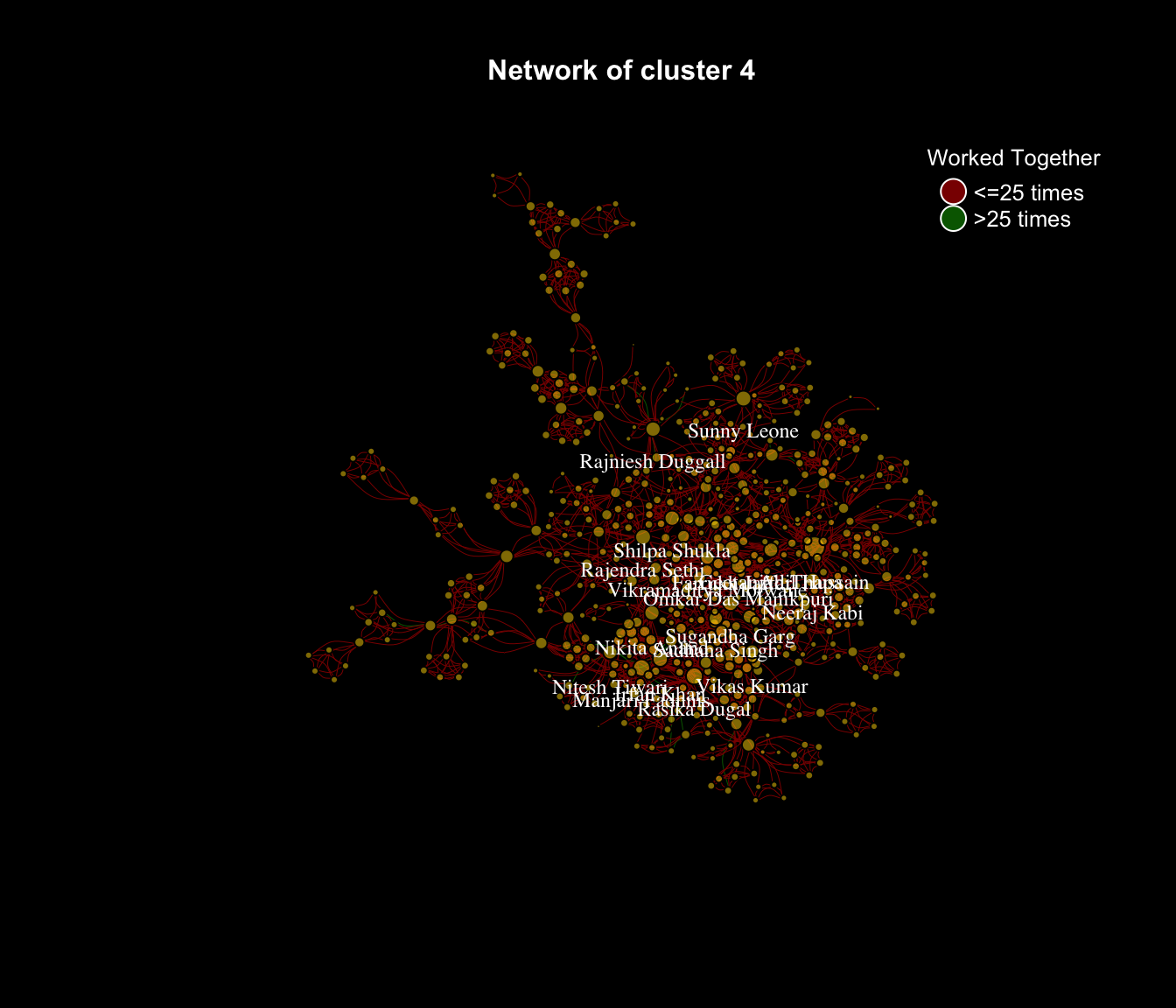 Central figure cannot be identified from this graph. There seems to be several who can clain to be 'central'. Eminent personality like Kamal Hassan, Girish Karnad, Smita Patil etc. are also present in this segment. Satyajit Ray and Anil Chatterjee too. Interestingly, they some of the major characters of parallel cinema.
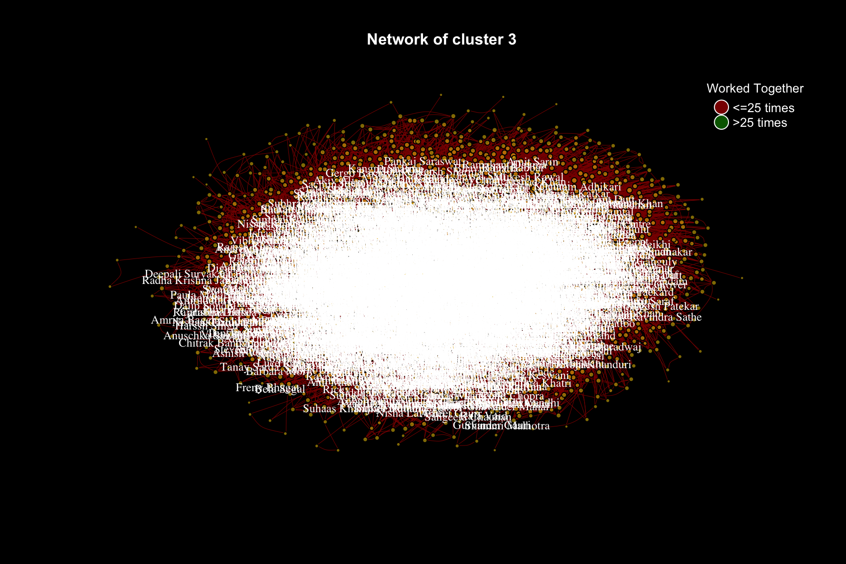
Mahabanoo Mody Kotwal seems to be the central figure in cluster 3. This group does not seem to consist of bollywood blockbuster creators. However, they have gained popularity in regional movies and television. Some of them are foreigners too.
 1comm.fg.3 <- as.undirected(induced_subgraph(gra.main, com.fg[[3]]))
 2
 3comm.fg.3.deg<-degree(comm.fg.3, mode = "all")
 4
 5
 6par(bg="black", mfrow=c(1,1))
 7plot(comm.fg.3,
 8     rescale= TRUE,
 9     vertex.label = ifelse(comm.fg.3.deg >= 11, names(V(comm.fg.3)), NA),
10     vertex.color = adjustcolor("gold", alpha.f = .5),
11     vertex.size = comm.fg.3.deg^(1/5),
12     layout = layout_with_lgl(comm.fg.3),
13     vertex.label.cex= 0.75,
14     vertex.label.degree=pi/2,
15     vertex.label.dist=1,
16     vertex.label.color="white",
17     edge.curved=0.5,
18     edge.width= 0.5,
19     edge.color = ifelse(comm.fg.3$weight>25, "dark green", "dark red"),
20     xlim = c(-1,1.1),
21     asp=-0.5)
22title("Network of cluster 3",cex.main=1,col.main="white")
23legend("topright", c("<=25 times",">25 times"), pch=21, col="white", pt.bg=c("dark red","dark green"), pt.cex=2, cex=.8, bty="n", ncol=1, title = "Worked Together", text.col = "white")
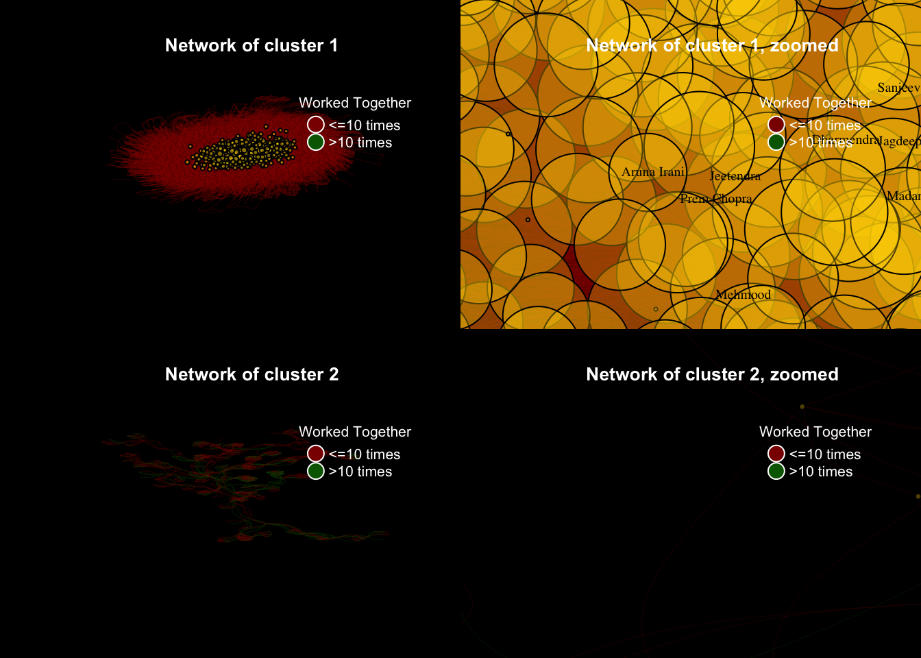
 Cluster 1 and 2 are too big and complex to show anything meaningful in the network plot. They need to be broken down further or other segmenting methods need to be used to capture different segments.
 1comm.fg.1 <- as.undirected(induced_subgraph(gra.main, com.fg[[1]]))
 2comm.fg.1.deg<-degree(comm.fg.1, mode = "all")
 3
 4comm.fg.2 <- as.undirected(induced_subgraph(gra.main, com.fg[[2]]))
 5comm.fg.2.deg<-degree(comm.fg.2, mode = "all")
 6
 7# cluster 1
 8par(bg="black", mfrow=c(2,2))
 9plot(comm.fg.1,
10     rescale= TRUE,
11     vertex.label = NA, #ifelse(comm.fg.2.deg >= 350, names(V(comm.fg.2)), NA),
12     vertex.color = adjustcolor("gold", alpha.f = .5),
13     vertex.size = ifelse(comm.fg.1.deg<50,0.1,(comm.fg.1.deg)^(1/4)),
14     layout = layout_with_lgl(comm.fg.1),
15     vertex.label.cex= 0.75,
16     vertex.label.degree=pi/2,
17     vertex.label.dist=1,
18     vertex.label.color="black",
19     edge.curved=0.5,
20     edge.width= 0.5,
21     edge.color = adjustcolor(ifelse(comm.fg.1$weight>10, "dark green", "dark red"),alpha=0.3),
22     xlim = c(-1,1.1),
23     asp=-1,
24     axes = F)
25title("Network of cluster 1",cex.main=1,col.main="white")
26legend("topright", c("<=10 times",">10 times"), pch=21, col="white", pt.bg=c("dark red","dark green"), pt.cex=2, cex=.8, bty="n", ncol=1, title = "Worked Together", text.col = "white")
27
28#cluster 1, zoomed
29plot(comm.fg.1,
30     rescale= TRUE,
31     vertex.label = ifelse(comm.fg.1.deg >= 350, names(V(comm.fg.1)), NA),
32     vertex.color = adjustcolor("gold", alpha.f = .3),
33     vertex.size = ifelse(comm.fg.1.deg<50,0.1,(comm.fg.1.deg)^(1/5)),
34     layout = layout_with_lgl(comm.fg.1),
35     vertex.label.cex= 0.75,
36     vertex.label.degree=pi/2,
37     vertex.label.dist=1,
38     vertex.label.color="black",
39     edge.curved=0.5,
40     edge.width= 0.5,
41     edge.color = adjustcolor(ifelse(comm.fg.1$weight>10, "dark green", "dark red"),alpha=0.2),
42     xlim = c(-0.025,0.025),
43     ylim = c(-0.025,0.025),
44     asp=-1,
45     axes = F)
46title("Network of cluster 1, zoomed",cex.main=1,col.main="white")
47legend("topright", c("<=10 times",">10 times"), pch=21, col="white", pt.bg=c("dark red","dark green"), pt.cex=2, cex=.8, bty="n", ncol=1, title = "Worked Together", text.col = "white")
48
49# cluster 2
50plot(comm.fg.2,
51     rescale= TRUE,
52     vertex.label = NA, #ifelse(comm.fg.2.deg >= 350, names(V(comm.fg.2)), NA),
53     vertex.color = adjustcolor("gold", alpha.f = .5),
54     vertex.size = ifelse(comm.fg.2.deg<50,0.1,(comm.fg.2.deg)^(1/4)),
55     layout = layout_with_lgl(comm.fg.2),
56     vertex.label.cex= 0.75,
57     vertex.label.degree=pi/2,
58     vertex.label.dist=1,
59     vertex.label.color="black",
60     edge.curved=0.5,
61     edge.width= 0.5,
62     edge.color = adjustcolor(ifelse(comm.fg.2$weight>10, "dark green", "dark red"),alpha=0.3),
63     xlim = c(-1,1.1),
64     asp=-1,
65     axes = F)
66title("Network of cluster 2",cex.main=1,col.main="white")
67legend("topright", c("<=10 times",">10 times"), pch=21, col="white", pt.bg=c("dark red","dark green"), pt.cex=2, cex=.8, bty="n", ncol=1, title = "Worked Together", text.col = "white")
68
69#cluster 2, zoomed
70plot(comm.fg.2,
71     rescale= TRUE,
72     vertex.label = ifelse(comm.fg.2.deg >= 350, names(V(comm.fg.2)), NA),
73     vertex.color = adjustcolor("gold", alpha.f = .3),
74     vertex.size = ifelse(comm.fg.2.deg<50,0.1,(comm.fg.2.deg)^(1/5)),
75     layout = layout_with_lgl(comm.fg.2),
76     vertex.label.cex= 0.75,
77     vertex.label.degree=pi/2,
78     vertex.label.dist=1,
79     vertex.label.color="black",
80     edge.curved=0.5,
81     edge.width= 0.5,
82     edge.color = adjustcolor(ifelse(comm.fg.2$weight>10, "dark green", "dark red"),alpha=0.2),
83     xlim = c(-0.025,0.025),
84     ylim = c(-0.025,0.025),
85     asp=-1,
86     axes = F)
87title("Network of cluster 2, zoomed",cex.main=1,col.main="white")
88legend("topright", c("<=10 times",">10 times"), pch=21, col="white", pt.bg=c("dark red","dark green"), pt.cex=2, cex=.8, bty="n", ncol=1, title = "Worked Together", text.col = "white")
Comparing the clusters
1l1<-mapping_monkey(comm.fg.1)
2l2<-mapping_monkey(comm.fg.2)
3l3<-mapping_monkey(comm.fg.3)
4l4<-mapping_monkey(comm.fg.4)
Comparing the histogram of degrees, betweenness and eigen vectors do not show any significant difference or unexpected outcome. In the histogram of eigen vectors of segment 3, the pattern is different from others. There are more individuals with higher eigen vectors. This is natural in a smaller group (Segment 3 is very small). People in a smaller group tend to connect to each other more than in those in larger group.
 1par(mfrow=c(3,4))
 2hist(l1[[1]], breaks = 50, col=adjustcolor("black", alpha=0.3), main = "Degrees, Segment 1", xlab = "Degrees")
 3hist(l2[[1]], breaks = 50, col=adjustcolor("red", alpha=0.3), main = "Degrees, Segment 2", xlab = "Degrees")
 4hist(l3[[1]], breaks = 50, col=adjustcolor("green", alpha=0.3), main = "Degrees, Segment 3", xlab = "Degrees")
 5hist(l4[[1]], breaks = 50, col=adjustcolor("blue", alpha=0.3), main = "Degrees, Segment 4", xlab = "Degrees")
 6hist(l1[[2]], breaks = 50, col=adjustcolor("black", alpha=0.3), main = "Betweenness, Segment 1", xlab = "Betweenness")
 7hist(l2[[2]], breaks = 50, col=adjustcolor("red", alpha=0.3), main = "Betweenness, Segment 2", xlab = "Betweenness")
 8hist(l3[[2]], breaks = 50, col=adjustcolor("green", alpha=0.3), main = "Betweenness, Segment 3", xlab = "Betweenness")
 9hist(l4[[2]], breaks = 50, col=adjustcolor("blue", alpha=0.3), main = "Betweenness, Segment 4", xlab = "Betweenness")
10hist(l1[[3]], breaks = 50, col=adjustcolor("black", alpha=0.3), main = "Eigen vectors, Segment 1", xlab = "Eigen Vector")
11hist(l2[[3]], breaks = 50, col=adjustcolor("red", alpha=0.3), main = "Eigen vectors, Segment 2", xlab = "Eigen Vector")
12hist(l3[[3]], breaks = 50, col=adjustcolor("green", alpha=0.3), main = "Eigen vectors, Segment 3", xlab = "Eigen Vector")
13hist(l4[[3]], breaks = 50, col=adjustcolor("blue", alpha=0.3), main = "Eigen vectors, Segment 4", xlab = "Eigen Vector")
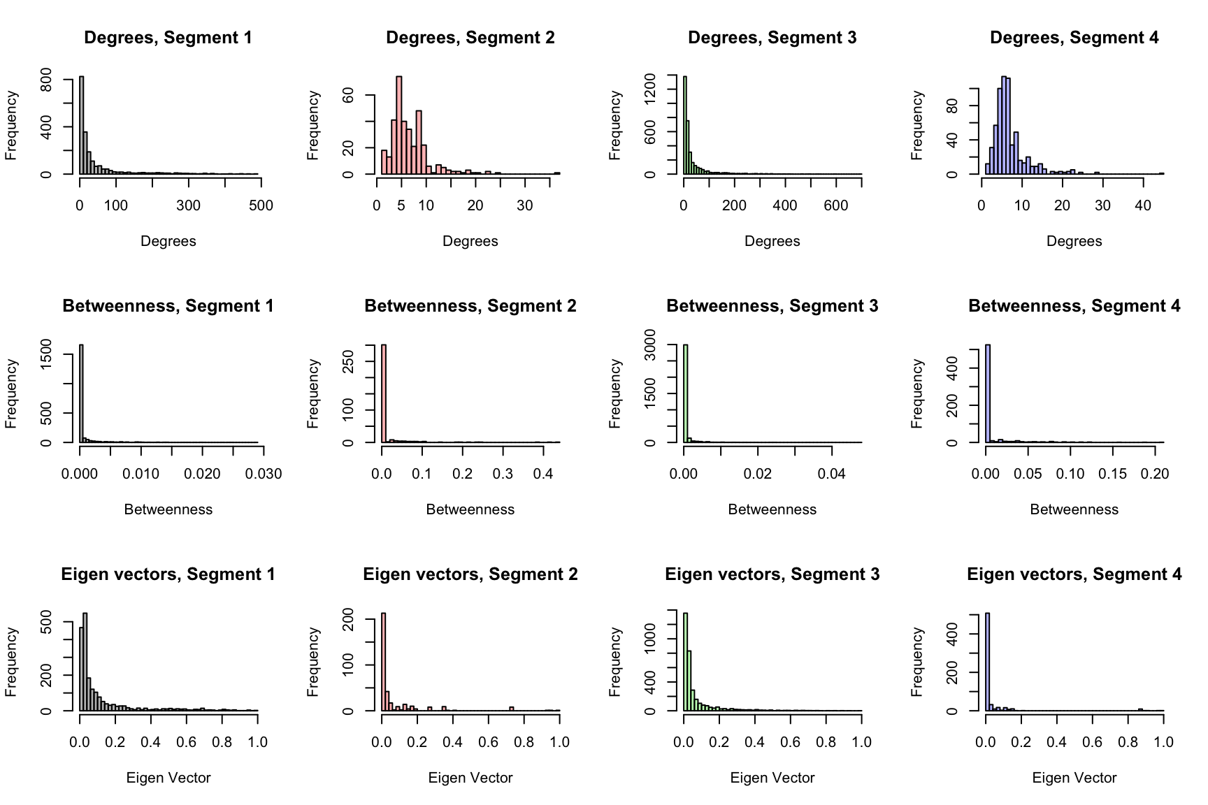
Variation in edge density is noticed in the segments. Segment 3, being smallest, can be expected to have higher density (people connected to each other). Comparing density of segment 2 and 4 is interesting. The population of segment 4 is much smaller. Yet, the density is lower than that of segment 2. This indicates that individuals in segment 2 are more connected (have worked with) to each other than those in segment 4. This, kind of, gets reinforced when the diameter is observed. The diameter of segment 4 is 8, compared to 4 of segment 2. This means that there are 3 connections in between the farthest points of the network in segment 2, compared to 8 in case of segment 4 (despite substantially lower population).
Another interesting observation is the assortativity of segment 3, which is highest. The tendency to stick together with people with similar number of connections is higher in segment 3.
1seg1<-c(l1[[4]],l1[[5]],l1[[8]],l1[[9]])
2seg2<-c(l2[[4]],l2[[5]],l2[[8]],l2[[9]])
3seg3<-c(l3[[4]],l3[[5]],l3[[8]],l3[[9]])
4seg4<-c(l4[[4]],l4[[5]],l4[[8]],l4[[9]])
5rname<-c("density", "diameter","assortativity", "transitivity")
6
7tba<-data.frame(`segmnt 1`= seg1,`segmnt 2`= seg2,`segmnt 3`= seg3,`segmnt 4`= seg4)
8rownames(tba)<-rname
9tba
1##                  segmnt.1    segmnt.2    segmnt.3     segmnt.4
2## density        0.02286444  0.02057270  0.01073862  0.012139805
3## diameter       5.00000000 13.00000000  5.00000000 12.000000000
4## assortativity -0.10422588 -0.03089446 -0.04228715  0.008327399
5## transitivity   0.21290278  0.21290278  0.21290278  0.212902779
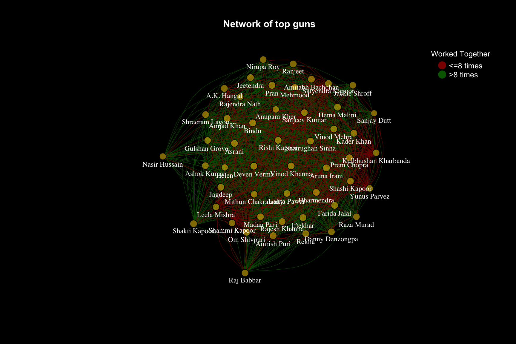
Final plot (for fun)
For fun, graph with individuals with highest eigen vector score is plotted to visualize the network among themselves.
 1ev<-sort(eigen.main$vector, decreasing = T)[1:50]
 2ename<-c(names(ev))
 3n<-c(match(ename,V(gra.main)$name))
 4
 5rock<-induced_subgraph(gra.main,vids=n)
 6rock.d<-degree(rock,mode = "all")
 7par(bg="black")
 8plot(rock,
 9     rescale= TRUE,
10     vertex.label = ifelse(rock.d >= 11, names(V(rock)), NA),
11     vertex.color = adjustcolor("gold", alpha.f = .5),
12     vertex.size = ifelse(rock.d<10,0.1,sqrt(rock.d)),
13     layout = layout_with_lgl(rock),
14     vertex.label.cex= 0.75,
15     vertex.label.degree=pi/2,
16     vertex.label.dist=1,
17     vertex.label.color="white",
18     edge.curved=0.5,
19     edge.width= 0.5,
20     edge.color = adjustcolor(ifelse(rock$weight>8, "dark green", "dark red"),alpha=0.9),
21     xlim = c(-1,1),
22     #asp=-1,
23     axes = F)
24title("Network of top guns",cex.main=1,col.main="white")
25legend("topright", c("<=8 times",">8 times"), pch=21, col="black", pt.bg=c("dark red","dark green"), pt.cex=2, cex=.8, bty="n", ncol=1, title = "Worked Together", text.col = "white")
This analysis can be further extended. Esp, by using clustering algorithms other than fast greedy. Moreover, detailed analysis of ego graphs may reveal interesting insights. Don't forget to share your results, if you do any of it.
Contact me if
- You want to understand how network analysis can help in your sales and marketing efforts.
- You are looking to collaborate for some investigation/research.