Optimization in R - purchase optimization to minimize cost

This article showcases solving an assumed business problem using optimization, with R as the tool to do so. Optimization problems come is various shapes and sizes and complexities. In this article the focus is on a simplified version of a problem to decide on purchase quantities to minimize cost. You may also like to read other examples of optimization series.
Introduction
Business units often must decide on purchase quantities under various constrains, to minimize cost. Mathematics can help with such decisions, as shown below using a simplified example.
Problem
XYZ corp is local supplier of milk. Having known the market for substantial amount of time, they have already developed a robust forecasting model. For the upcoming days, they expect the following demand.
| Day | 1 | 2 | 3 | 4 |
|---|---|---|---|---|
| Demand (l) | 5000 | 8000 | 9000 | 6000 |
They need to purchase milk from suppliers at market prices every day. They also have a refrigerated tank that can hold 4000 l of milk. The daily price is expected to be as follows.
| Day | 1 | 2 | 3 | 4 |
|---|---|---|---|---|
| Price ($/l) | 0.75 | 0.72 | 0.92 | 0.90 |
Their current stock is 2000 l. XYZ wants to purchase milk everyday (at the beginning of the day) to satisfy customer demand at minimal cost. The milk is delivered directly to customer and only the leftover of the day is stored in the tank.
Solution
Objective function
The function of margin can be defined as
\(m_n\) is the quantity of milk to purchase.
Constrains
If the tank already contains \(t_1\) milk at the beginning of day 1 and XYZ buys \(m_1\) liters on that day, it should cover the demand of that day (5000 in this case for day 1) and the remaining needs to be stored in the tank. This becomes the initial stock of day 2 or \(t_2\).
The second and third lines are rearrangement of the first line to help us construct the matrix. But, we also know that \(t_1\) is 2000. So the equation becomes
Following the same logic, we also have
Also,
Because purchase of day 4 and stock at the beginning of the day should satisfy the demand of the day.
Finally,
Solving the equations
 1library(lpSolve)
 2
 3objective.fn <- c(0.75, 0.72, 0.92, 0.90, 0, 0, 0)
 4const.mat <- matrix(c(1, 0, 0, 0, -1, 0, 0,
 5                      0, 1, 0, 0, 1, -1, 0,
 6                      0, 0, 1, 0, 0, 1, -1,
 7                      0, 0, 0, 1, 0, 0, 1,
 8                      0, 0, 0, 0, 1, 0, 0,
 9                      0, 0, 0, 0, 0, 1, 0,
10                      0, 0, 0, 0, 0, 0, 1,
11                      1, 0, 0, 0, 0, 0, 0,
12                      0, 1, 0, 0, 0, 0, 0,
13                      0, 0, 1, 0, 0, 0, 0,
14                      0, 0, 0, 1, 0, 0, 0,
15                      0, 0, 0, 0, 1, 0, 0,
16                      0, 0, 0, 0, 0, 1, 0,
17                      0, 0, 0, 0, 0, 0, 1
18                      ) , ncol=7 , byrow=TRUE)
19
20const.rhs <- c(3000, 8000, 9000, 6000, 4000, 4000, 4000, 0, 0, 0, 0, 0, 0, 0)
21const.dir <- c("=", "=", "=",">=","<=","<=","<=", ">=",">=",">=",">=",">=",">=",">=")
22lp.solution <- lpSolve::lp("min", objective.fn, const.mat,
23                  const.dir, const.rhs, compute.sens=TRUE)
24lp.solution$solution
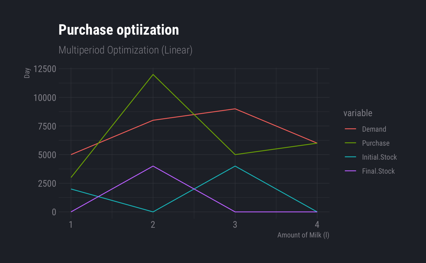
Hence, the optimum solution to minimize cost under the given condition is to order 3000, 12000, 5000 and 6000 liters of milk for the respective days. This cost will then be 20890 dollars.
Insights
Optimum purchase quantities are as follows
| Day | Purchase (liters) | Demand/Sales (liters) | Initial Stock (liters) | Final Stock (liters) |
|---|---|---|---|---|
| 1 | 3000 | 5000 | 2000 | 0 |
| 2 | 12000 | 8000 | 0 | 4000 |
| 3 | 5000 | 9000 | 4000 | 0 |
| 4 | 6000 | 6000 | 0 | 0 |
The optimum values will not change within these following price ranges.
1data.frame(Price=c("Day 1","Day 2", "Day 3", "Day 4"), From=round(lp.solution$sens.coef.from[1:4],2), To=round(lp.solution$sens.coef.to[1:4],2))
1##   Price     From      To
2## 1 Day 1  7.2e-01 1.0e+30
3## 2 Day 2 -1.0e+30 7.5e-01
4## 3 Day 3  9.0e-01 1.0e+30
5## 4 Day 4  0.0e+00 9.2e-01
Furthermore, the following table shows the possible change in objective function (i.e. cost) on relaxing the constrain i.e. the demands each day. In this case, if demand is relaxed by one unit, the change in cost function is shown.
Posts in this Series
- Optimization in R - purchase optimization to minimize cost
- Optimization in R - Production quantities to maximize profit