Everyone knows how annoying mechanical breakdown can be. Production is directly successful because the equipment malfunctions. Large sums of money are lost as production resumes. It also affects OEMs and distributors based on lost reputation and business opportunity. Fortunately, the use of data science can handle this problem to a large extent.
Opportunity for machine owners
The cost of breakdown is not only the loss of opportunity (profit from production), but also the fixed cost of the machine. Also, delays in production can attract fines and lost orders. Sometimes, while other machines depend on failed machines, the cost increases through the roof. The cost of a single break can easily exceed thousands of dollars. The worst part is that this loss can never be recovered.
The figure above shows some of the components of cost of downtime.
Using predictive models, one can now estimate the probability of failure. It gives us two abilities. First, the ability to plan maintenance to minimize losses. Second, to improve inventory better. Instead of stockpiling a lot of spare parts, it is possible to keep only what you need in the future.
Advantages for machine owners
- Reduce repair time
- Avoid unplanned maintenance
- Reduce inventory cost
- Increase bottom line
Opportunity for manufacturers (OEMs)
Failures do not directly affect OEM, but it can damage reputation and end up in lost business. If an important item is not available nearby, customers will not hesitate to purchase items from the local market. Also, manpower may not be available to repair the machine immediately.
These problems can be avoided if you already have an idea of the potential breakdowns. OEMs / Distributors can then schedule a maintenance and replace parts or provide immediate support in the event of a breakdown. In addition, it will enable OEMs to introduce new revenue models of maintenance contracts. It can also ensure that customers do not buy spare parts from local markets.
Advantages for OEMS
- Avoid unplanned breakdowns
- Increase customer satisfaction (lower repair time)
- Optimize inventory
- Improve top line
- Improve product
How to implement
The process begins by identifying the problems to be solved. Usually the problem should be broad and exclusively segregated. E.g. The goal may be to reduce operating costs. One of the many ways to achieve this is by reducing idle time and improving the list of spare parts.
Once problems are identified, data should be collected for analysis. Often data is not available. As such, the infrastructure for data collection needs to be built. When creating infrastructure and processes, efforts should be made to improve the utility of such infrastructure / processes. This can be done by evaluating other uses of the collected data. If it costs somewhat less to add additional data to solve a significant problem, it should proceed.
Once the data starts to collect, it should be cleaned and visualized. This applies not only to the data science team, but also to other business partners. If possible and possible, the dashboard (s) can be built for different partners depending on the need. Predictive features of analyzes are natural advances from research analyzes. Dashboards and visualization should be tested and reviewed by creating a forecast model (s).
Example using real life data
Code heavy!!! Skip if you are not interested in the codes. However, you may like to understand how well the below model performed in results
Real life (normalized) data have been used to illustrate the possible model. The data contains a record of certain parameters taken per hour. In addition, record and maintenance of failures will be used. 1 The parameters recorded in hours are voltage, vibration, rotation and pressure. Data were recorded from 100 machines of 4 types. Failure of 4 components has been recorded. To simplify, let us analyze the failure of ‘comp2’.
To keep this brief and to focus on the prognostic model many research activities have been avoided.
Code
# Following data are available
# 1. Telemetry - Logs hourly parameters (Voltage, Pressure, Rotation and Vibration) for each machine
# 2. Failures - Log of component failures. Contains the time slot (that matches the telemetry log) and machineID
# 3. Maint - Log of maintainance. Contains time slot, machineID and the component replaced
# 4. Assets - Information about the machines - machineID, Model and age

# Function to calculate number of periods since last maintenance of a component
timeslm <- function(k) {
  output <- c()
  output[1] = 0
  for (i in 2:length(k)) {
    if (k[i - 1] == 1) {
      output[i] = 1
    } else {
      output[i] = output[i - 1] + 1
    }
  }
  return(output)
}

# For the sake of simplicity, failures of 'comp2' will be analysed

#preparing data
failures2 <-
  failures %>% filter(failure == "comp2") #new data frame with failure of comp2
maint2 <-
  maint %>% filter(comp == "comp2") #new data frame with maintenance of comp2

df <-
  telemetry %>% left_join(failures2, by = c("machineID", "datetime")) %>% #Joining log with failure
  mutate(failed = ifelse(is.na(failure), 0, 1)) %>%  #creating column with binary (failed or not)
  left_join(maint2, by = c("machineID" = "machineID", "datetime" = "datetime")) %>% #Joining maintenance data
  mutate(maint = ifelse(is.na(comp), 0, 1)) %>% #New column with binary (maintained or not)
  inner_join(assets, by = "machineID") #Joining machine details
df$datetime <-
  parse_date_time(df$datetime, "mdy HMS p") #Changing column type to date time
df$machineID <- as.factor(df$machineID)
df$model <- as.factor(df$model)

timesm <- timeslm(df$maint) #Calculating periods since maintenance
df$timesm <- timesm

df <-
  df %>% mutate(t = ifelse(is.na((
    as.numeric(datetime - lag(datetime, 1))
  )), 0, (as.numeric(
    datetime - lag(datetime, 1)
  )))) %>%
  mutate(tim = cumsum(t)) #Adding time columns

df <- df[, c(1, 14, 15, 13, 11, 12, 2:6, 8, 10)]
#Column details - datetime = event log time
#                 machineID = Machine Identification number
#                 volt, rotate, pressure, vibration are some of the parameters that are measured
#                 failed and maint indicate if the component (comp2) failed. 1 indicates true.
#                 age is the age of the machine
#                 timesm is the time since maintenance
#                 tim is the time since the beginning of event logging


#removing dfs that are not required
rm(telemetry)
rm(assets)
rm(failures)
rm(maint)
rm(timesm)

# adding grouping to calculate cumulative parameter values.
g <- c()
g[1] = 1
for (i in 2:nrow(df)) {
  if (df$timesm[i] < df$timesm[i - 1]) {
    g[i] = g[i - 1] + 1
  } else {
    g[i] = g[i - 1]
  }
}

df$group <- g

# removing unwanted data
rm(g)


#Will add new columns with cumulative parameters - sum, mean

df1 <-
  df %>% group_by(group) %>% mutate(
    volt.cum = cumsum(volt),
    vib.cum = cumsum(vibration),
    pres.cum = cumsum(pressure),
    rot.cum = cumsum(rotate),
    volt.mean = cumsum(volt) / seq_along(volt),
    vib.mean = cumsum(vibration) / seq_along(vibration),
    pres.mean = cumsum(pressure) / seq_along(pressure),
    rot.mean = cumsum(rotate) / seq_along(rotate)
  ) %>%
  filter(maint == 1)   # filtered required data

# In case you are interested to know about the transformations in detail please get in touch.

#preparing test and train data
df.train <- df1 %>% filter(datetime < "2015-11-15 06:00:00 UTC")
df.test <- df1 %>% filter(datetime > "2015-11-15 06:00:00 UTC")

#removing unwanted data
rm(df1)
rm(df)

# Fitting Kaplan Meier

kap.fit<-survfit(Surv(timesm,failed)~model, data=df.train)

#Plotting

fig<-ggsurvplot(
  kap.fit,
  pval = F, # show p-value
  break.time.by = 1000, #break X axis by 25 periods
  #risk.table = "abs_pct", # absolute number and percentage at risk
  #risk.table.y.text = FALSE,# show bars instead of names in text annotations
  linetype = "strata",
  # Change line type by groups
  conf.int = T,
  # show confidence intervals for
  #conf.int.style = "step",  # customize style of confidence intervals
  #surv.median.line = "hv",
  # Specify median survival
  ggtheme = theme_minimal(),
  # Change ggplot2 theme
  legend.labs =
    c("Model 1", "Model 2", "Model 3", "Model 4"),
  # change legend labels
  ncensor.plot = F,
  # plot the number of censored subjects (outs) at time t
  #palette = c("#000000", "#2E9FDF","#FF0000")

)+
  labs(x="Hours")
fig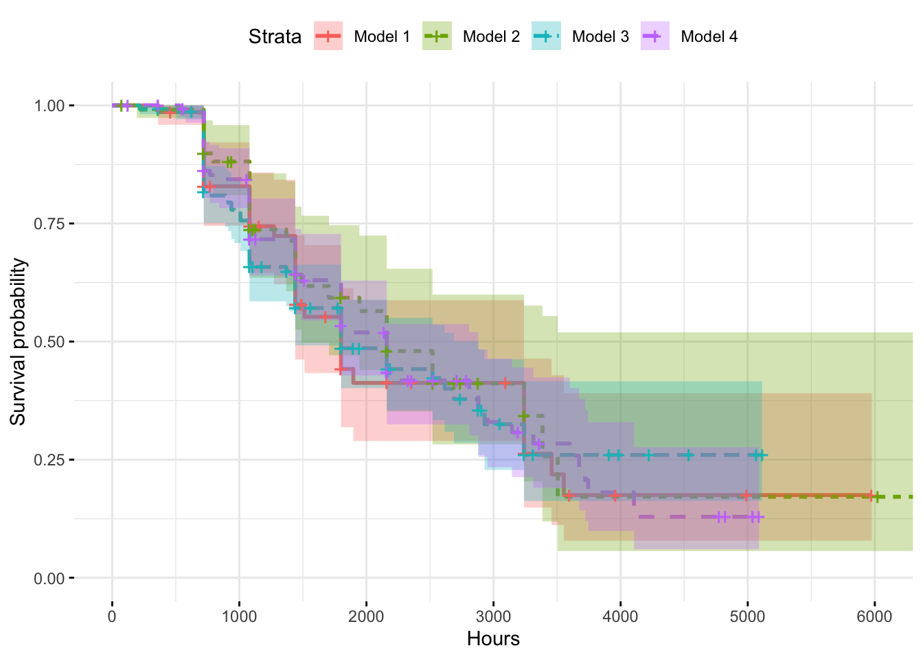
Kaplan Meier model predicts survival chances by 3000 hours of operation (post maintenance) reduces significantly. But there is a substantial amount of uncertainty in prediction, except in case of model 4. The model also shows that it is almost certain that there will be no failures till about 700 hours of operation, post maintenance.
Summary of the fit is as shown below.
Code
summary(kap.fit)$table records n.max n.start events rmean se(rmean) median 0.95LCL
model=model1 103 103 103 37 2661.662 317.7212 1800 1440
model=model2 112 112 112 32 2781.430 370.7489 2160 1489
model=model3 257 257 257 78 2871.243 264.5345 1800 1440
model=model4 191 191 191 70 2620.189 214.6314 2160 1800
0.95UCL
model=model1 3240
model=model2 NA
model=model3 2880
model=model4 2880Since the uncertainty is high, I will not use this model and try Cox regression.
Cox regression model shows that among all the parameters used, cumulative rotation is the one that significantly impacts failure of ‘comp2’.
With this insight, OEM can think of ways to improve component quality or find out ways to keep the rotation low.
Code
# Cox regression
cox.fit<-coxph(Surv(timesm,failed) ~ volt.cum+vib.cum+pres.cum+rot.cum+volt.mean+vib.mean+pres.mean+rot.mean+factor(model), data=df.train)
summary(cox.fit)
Call:
coxph(formula = Surv(timesm, failed) ~ volt.cum + vib.cum + pres.cum +
rot.cum + volt.mean + vib.mean + pres.mean + rot.mean + factor(model),
data = df.train)
n= 663, number of events= 217
coef exp(coef) se(coef) z Pr(>|z|)
volt.cum -2.389e-04 9.998e-01 1.416e-04 -1.687 0.091529 .
vib.cum -3.233e-04 9.997e-01 2.849e-04 -1.135 0.256382
pres.cum 2.164e-05 1.000e+00 1.557e-04 0.139 0.889459
rot.cum -1.496e-04 9.999e-01 4.161e-05 -3.594 0.000326 ***
volt.mean 2.527e-01 1.287e+00 1.687e-01 1.498 0.134178
vib.mean 5.436e-01 1.722e+00 3.291e-01 1.652 0.098603 .
pres.mean 1.520e-01 1.164e+00 1.851e-01 0.821 0.411487
rot.mean -4.229e-02 9.586e-01 4.338e-02 -0.975 0.329642
factor(model)model2 -4.183e-01 6.582e-01 2.786e-01 -1.501 0.133273
factor(model)model3 -1.932e-01 8.243e-01 2.322e-01 -0.832 0.405304
factor(model)model4 9.385e-02 1.098e+00 2.397e-01 0.391 0.695429
---
Signif. codes: 0 '***' 0.001 '**' 0.01 '*' 0.05 '.' 0.1 ' ' 1
exp(coef) exp(-coef) lower .95 upper .95
volt.cum 0.9998 1.0002 0.9995 1.0000
vib.cum 0.9997 1.0003 0.9991 1.0002
pres.cum 1.0000 1.0000 0.9997 1.0003
rot.cum 0.9999 1.0001 0.9998 0.9999
volt.mean 1.2875 0.7767 0.9250 1.7920
vib.mean 1.7222 0.5807 0.9035 3.2826
pres.mean 1.1641 0.8590 0.8100 1.6731
rot.mean 0.9586 1.0432 0.8804 1.0437
factor(model)model2 0.6582 1.5193 0.3813 1.1363
factor(model)model3 0.8243 1.2132 0.5229 1.2994
factor(model)model4 1.0984 0.9104 0.6866 1.7571
Concordance= 0.98 (se = 0.004 )
Likelihood ratio test= 1060 on 11 df, p=<2e-16
Wald test = 135.2 on 11 df, p=<2e-16
Score (logrank) test = 483.9 on 11 df, p=<2e-16So, a new model was built to include only cumulative rotation as parameter. The model was used to predict outcome on test data. Confusion matrix was built to analyze accuracy.
Code
# Revised cox model
cox.fit<-coxph(Surv(timesm,failed) ~ rot.cum, data=df.train)

# Predicted probabilities
pred<-predict(cox.fit,newdata=filter(df.test), type = "expected")

d<-df.test%>%cbind(pred=pred)%>%select(12,14,23)%>%mutate(pred=ifelse(pred>0.5,1,0))

table(act=d$failed,pred=d$pred)
pred
act 0 1
0 49 12
1 7 32Results
- 81 % accuracy was achieved *
- 87 % accurate when did not predict failure *
- 72 % accurate when predicted failure *
Wondering what does it mean in terms of saved cash? Or what are all possible ways to create value out of this? One needs more detail of the business and operations to answer those questions. If you are really interested, you know what to do!
For any questions and/or clarifications, please do not hesitate to contact me.
Notes
Footnotes
The data has been sourced from [Deepti Chevvuri’s Github] (https://github.com/DeeptiChevvuri/Predictive-Maintenance-Modelling-Datasets). The data contains error logs as well, which has not been used in this analysis.↩︎